-
-
-
-
URL copied!

Welcome back to my three-part blog series, discussing Data Parallelism and Distributed Deep Learning at production scale.
In part one, I discussed how we at GlobalLogic approach serverless data processing at scale using Amazon Web Services (AWS), if you haven’t read it yet you can read it here! However, if you are a Machine Learning (ML) enthusiast and want to skip to the distributed deep learning bits, then get your popcorn ready and continue reading for part two.
Today, we’re talking ML taboo… you guessed it, cost!
There are two primary costs in ML, first being ‘financial cost’ and second ‘carbon burden’.
Considering carbon burden, companies are investing heavily into sustainable solutions to reduce their carbon impact on the environment. However regarding financial cost, whilst many companies have indeed achieved incredible reductions in operating costs by optimising infrastructure around ML, few have invested into distributed ML (data-parallel or model-parallel)– offering significant gains in efficiency and a reduction in cost. Here at GlobalLogic we have achieved these cost reductions, carbon emission reduction and more!
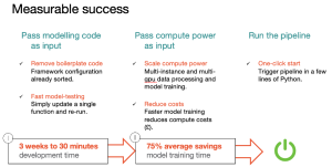
The examples in this blog series are productionised using our in-house bespoke Deep Learning accelerator service offering. If your company require Deep Learning models for life (not just for Christmas) then get in touch and we’ll be happy to help!
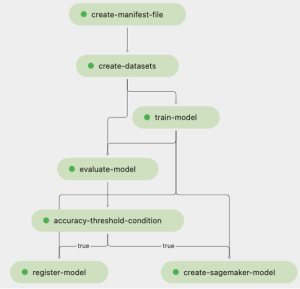
Figure 1 SageMaker Training Pipeline
Note: This blog only contains snippets of SageMaker Pipelines code, not the full scripts. The purpose of this blog series is to provide guidance and links to helpful resources.
Our distributed deep learning high-level design
By the end of this second blog, I will have created a SageMaker Pipeline to handle distributed ML in two pipeline steps:
- Create training job
- Evaluate model performance
The first step is where most of the magic happens, so I’ll spend much of this article discussing this step. At a very high level, I have created the following design to help visualise the model training step for a holistic point-of-view:
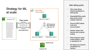
Figure 2 High-Level Design for Distributed Deep Learning
Note: this design is the tip of the iceberg. If we’re giving away these game-changer designs for free, imagine what more we aren’t showing!
Distributed learning reduces your carbon footprint
Before we dive into the blog’s main course, it is worth having a starter on why distributed computing is so important. There has been a troubling trend in recent years and a 2019 study found ‘the average deep learning model can generate up to 626,155 pounds of CO2 emissions’ – roughly equal to the total lifetime carbon footprint of five cars.
As models are becoming more complex, compute resources are getting cheaper and there is a recent trend towards huge inter-connected modelling solutions (Artificial General Intelligence).
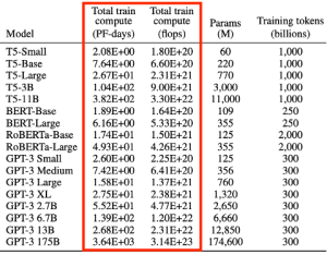
Figure 3 OpenAI’s GPT3 models took a sum of 4,156 days (11.4 years) or 552 metric tons of carbon to train.
While Deep learning has undoubtedly done a lot of good for climate sustainability, a lack of thought leadership towards carbon optimisation within the commercial sectors has resulted in incredibly wasteful ML systems.
At GlobalLogic, our mission is ‘Sustainable Product Engineering’ – so when considering our MLOps architecture designs we ensure max utilisation of all our compute resources as well as knowing when to turn off the lights (quite literally).

Figure 4 Stretching compute utilisation to the limit using intelligent scaling
Machine Learning at production scale
There are many ways to ‘productionise’ code. Few of them are correct.
It is exceptionally difficult to put models into production because it requires the collaboration of many entirely different skillsets. Data scientists often write their code in (messy) Jupyter notebooks which are excellent tools for exploration but are not scalable into production. Also, many of us Data Scientists are not experts in Continuous Integration, Continuous Deployment (CI/CD) pipelines.
Software engineers and DevOps alike are versatile with their tools and have high coding standards, but might not be used to dealing with uncertainty – which is an integral part of Machine Learning.
Also, as Solutions architects and application developers aren’t used to what modelling inputs and outputs look like, there can be difficulty when fitting the model into architecture designs. This can lead to uncertainty when deciding what infrastructure is required for creating well-architected, fault-tolerant systems.
While we don’t have time to discuss all those issues. It’s important to realise that data scientists cannot, or rather should not productionise ML models alone – we need help!
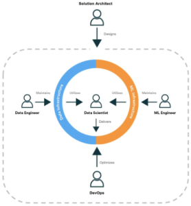
Figure 5 Data scientists need to communicate effectively with other teams
After wrapping your head around the complexities of team structures, the model training part is easy! So, let’s crack on to training our models…
Now, bear with us, this bit gets a little technical – but then again, we are talking about tech so this shouldn’t be a surprise!
Step 1: Create the training job
The training job consists of two parts:
- Create a SageMaker Pipelines training step
- Write the training code
Step 1.1: Create a SageMaker Pipelines training step
If you remember back to our processing step, we created many ‘*.tfrecord’ files. Now we need to tell our training job to use the generated files by providing our training job a dictionary of S3 URIs (mapped to each one of our training, validation, and testing channels). If like me, you like to keep things simple you can use the same number of *.tfrecord files as the number of GPUs you have available. Like so:
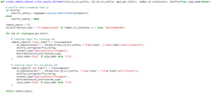
Figure 6 dynamically generate remote inputs with configurable ingestion parameters
Let me explain a few things.
FullyReplicated essentially means all the data will be copied to each compute instance we use. A single compute instance can contain multiple GPUs. Each GPU will have access to the entirety of the data.
ShardedByS3Key means the data will be automatically split between multiple instances. Therefore, ‘algo-1-train.tfrecord’ will be available to n-training-instances, and each training-instance will have samples like the below:

Pipe Mode means the data will be streamed to each instance. This allows your training job to run almost immediately without waiting for all the data to download first. I find on average this saves approximately 3-4 minutes of training time (of course dependent on the file/s size) and can be very helpful when initially making sure the training script runs without errors.
In most scenarios you will not need access to all the data before starting training (because usually you will train on small batches of data at a time anyway) – provided you apply data transformations on the fly (in mini-batches). To make SageMaker training aware your data will be a ‘streaming body’ you need to cast your dataset with SageMaker’s PipeModeDataset class.
File Mode is the default input mode option. Using this option, the training job will download the file from S3 in its entirety before the training script is executed. This option is the most straightforward but will delay your training job from starting – incurring SageMaker Training costs before training even begins.
For example, let’s say we use two training compute instances and our reason for doing so is because we have a lot of training data, and we need to decrease training time. In this scenario, the appropriate distribution type is ‘ShardedByS3Key’ because we want each instance to be working on only half the training samples.
Each instance will have access to the same file names however, the file sizes will simply be halved. From the user’s perspective, the code doesn’t require any changes and they can expect to have access to the same file directory structure.
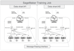
Figure 7 High-level design of multi-instance, multi-GPU distributed training
Next step is to specify the training job parameters. At production, the training parameters dictionary should be dynamically generated but, to keep things simple, we’ll keep the dictionary static for now.
To use distributed training, we need to specify the ‘distribution’ parameter (as shown in figure 8). In our example we are using Message-Passing-Interface (MPI), a commonly used message-passing system that is standard in many parallel computing architectures and provides a reliable architecture for High-Performance Computing (HPC).
Another distribution strategy we could have used is SageMaker’s own message-passing system ‘smdistributed’ that has been further optimised to run on AWS resources; however, at the time of writing, this distribution strategy can only be used with the following (very large, very expensive) instance types: "ml.p4d.24xlarge", "ml.p3dn.24xlarge", and "ml.p3.16xlarge". The number of processes (GPU or CPU cores) need to be known in advance.
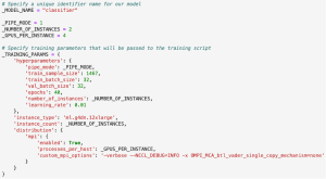
Figure 8 Example of training job parameters
Next, we need to create the TensorFlow SageMaker estimator. A SageMaker estimator object essentially sets out the configuration for model training. Our estimator (shown below) will also automatically track training metrics using regular expressions and we can later view/ query these metrics using Amazon Cloudwatch.
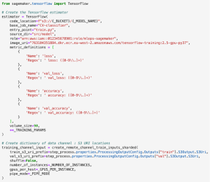
Figure 9 Create estimator for our training job
Finally, we create the training job step, passing our estimator and training input channels as arguments. At the time of writing, there is a bug with the estimator input mode where this can revert to the default ‘File’ mode. So, I manually update the input mode of the estimator after creating the training step variable.
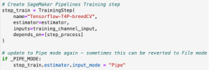
Figure 10 Create training job step
Step 1.2: Write the training code
Sadly, it is a common misconception that you can only use black-box models on SageMaker. (The term ‘black-box’ means the inputs and outputs are seen and the code being executed is hidden). This is far from the truth. Only the algorithms owned by Amazon are black-box models and even then, there is enough documentation to make an educated guess on how they have been developed.
All the commonly used open-source frameworks that appear to be black-box models have their code available on public GitHub repos, so you can see the implementation and how they work. In the past, many of my clients have strayed away from using Amazon for model development because they wrongly believe it isn’t malleable for their ‘unique’ use-case – only to transition to alternative third-party ML platforms (AutoML solutions) that are more-often-than-not black-box models.
For example, one of my previous clients spent six months investing in new third-party technology because they did not know SageMaker provided an out-of-the-box option for Hyper-Parameter Tuning and cross-validation for specifically XGBoost models. A five-minute Google search would have saved them six months of development time and millions of pounds investment.
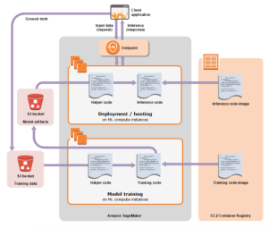
Figure 11 SageMaker provides Bring-Your-Own-Model (BYOM) architecture
In our example for distributed training, we do not need to create our own containerised docker image (‘Training code image’, figure 11). There are already docker images available for both training and inference of Tensorflow models as well as other deep learning frameworks.
I always suggest using the readily available images where possible, as these come pre-installed with some additional features such as automatically configuring MPI, Multi-Model-Server (MMS) deployment, TensorFlow Serving, TFX and model compilation and many more. With the docker image already created the only thing we need to worry about is the entry is our training code.
Both the Horovod and openMPI packages are pre-installed on the docker images we are using, so we can simply import these packages and start using them! There are Horovod implementations for other common Deep Learning frameworks too and SageMaker provides pre-built Docker containers for the most common ones (E.g., PyTorch and Apache MXNet).
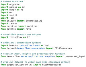
Figure 12 Import common utility functions, Tensorflow and Horovod
After our imports, we need to configure our training environment and set some global variables (ideally, these global variables would be passed to our training environment instead of being defined statically).
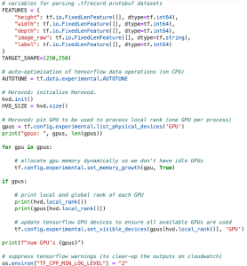
Figure 13 Create global variables and initialise Horovod
Next, we introduce some more functions. We need functions for parsing the protobuf ‘.tfrecord’ datasets, processing our input and lastly, a function for defining our neural network architecture. I’ve included some basic example code snippets for these steps below:
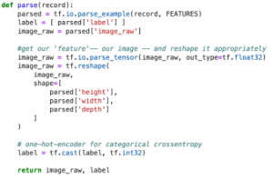

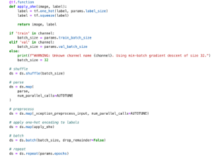
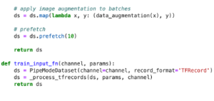
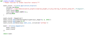
In this example we are using an open source pretrained computer vision model (from ImageNet). These model weights could be passed to our training job using file mode, or we can download them inside the training job execution (provided the training job has internet access). I always advise limiting the internet access of your training job to avoid security issues.
Finally, we write the main code block. This code block is executed when the Python training script (i.e., ‘entrypoint’ executable) command is ran in our Docker image.
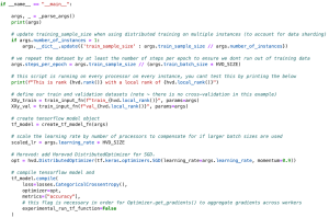
Let’s digest what’s happening so far.
When training neural network models, we need to know how many training samples we have per epoch. An epoch is one full cycle of training data. So, if we need to train for several epochs (i.e., train on the data samples more than once) then we need to repeat our dataset for that many epochs.
However, because we have chosen to use multiple training instances, we have split the number of training samples between each instance, so we need to update our script to account for this. We can either pass the number of instances as a parameter to our training script (as shown in the example) or we can access this information within the ‘resourceConfig.json’ file that’s created dynamically when creating the training job. We use the number of training samples to figure out how many steps there are per epoch.
It’s important to reiterate this script is run on every processor. Therefore, when loading the data, you will notice each GPU is accessing a unique subset of the data (indexed by the GPU local_rank). Multiple GPU’s will have the same local rank if more than one compute instance is used, however as the dataset is initially sharded between multiple instances, the data files, which each GPU is accessing, will have different content for every compute instance.
We scale the learning rate by the number of processors to account for a larger batch size. This is an optional step; however, the training will be more efficient if using larger batch sizes (as this helps prevent bottlenecks when processors wait for one another to finish). An increase in learning rate will help speed-up optimising model weights (backpropagation), helping negate the reduction in training steps when using a larger batch size.
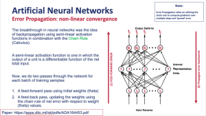
Figure 14 Summary of how neural networks learn
Lastly, our optimiser is wrapped by Horovod’s implementation for distributed optimisation (which handles the all-gather and all-reduce MPI operations).
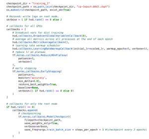
We next assign training callbacks to GPU processors based on the processor’s (unique) global rank. By default, rank-0 is designated as the root node. There are some operations we only need executing on a single node (for example, using a model checkpoint to save model weights to file).
Each processor will effectively run their own training job which optionally prints training accuracy, loss, and custom metrics to CloudWatch. To prevent being inundated by output metrics, we only allow the root node to print training progress, as well as the averaged accuracy/error at the end of each epoch.
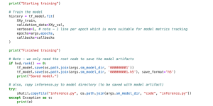
Finally, we simply fit the model with our training and validation datasets. All processors will each start their own training job, and (by default) after every epoch each processor will communicate, to the root node the model parameters that gave the best model accuracies. The root node will calculate the mean average of all model weight updates and will then broadcast these averaged model parameters to all GPU processors.

In a very small amount of code, we can now create Deep Learning models using distributed training – massively decreasing our training time and cost.
In this blog we’ve discussed the tip of the iceberg of what optimisation options are available to you however, Horovod have a lot more great functions you can take advantage of to further optimise training your ML models.
Step 2: Evaluate the model
All models created by data scientists need to be tested against unseen data to prove they perform as expected when released into production. This is called the evaluation (or testing) step. In this step we invoke our model with the subset of data we previously set aside in our processing step (the testing dataset).
Note: we could include model testing in our training script but it’s good practice to follow a separation-of-concerns software design pattern.
Step 2.1: Create a SageMaker Pipelines evaluation step
I won’t go into too much detail for this step as it is straightforward. Essentially, we just need to create another SageMaker Processing job that accepts the testing dataset as input, processes this dataset (applying the same processing functions as when processing the train and validation datasets), loads and invokes our newly trained model and returns model metrics.
To do this, we create another SageMaker Pipelines processing step and attach an evaluation python script. We pass the model artifact that was produced at the end of our training job as well as optionally passing a ‘PropertyFile’. This property file allows us to write our evaluation metrics to a JSON file – which we will later pass to a conditional threshold step in part three of this blog series!
We don’t need to use distributed processing for this step as the evaluation is only a single epoch. We can quite easily do this using a single, less powerful compute instance. If you have millions of samples needing inference (for example, perhaps inferencing artificially generated samples) then you could repeat the data sharding steps I shared in part one of this blog series and split the testing data over several compute instances.
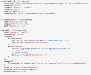
Figure 15 Example SageMaker Pipelines evaluation step
Step 2.2: Write the evaluation code
The evaluation code does not need to be complex. I’ve included an extra snippet of code here to allow for the user to select which model version/s to evaluate.
For those who are thinking several steps ahead, we don’t have to train and save only one model. If you were so inclined, you could expand distributed training to perform more time-consuming efforts such as performing cross-validation across multiple processors in a single training job, training several models with different neural network architectures to find the best performing architecture or creating your own variant of an AutoML solution.
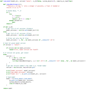
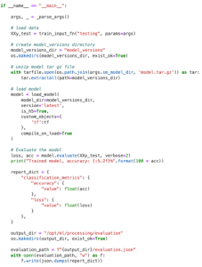
Figure 16 Example testing script
And that’s it! We can test our pipeline by running the following code:
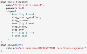
Figure 17 Execute the SageMaker Pipeline
You can test this is working by looking at the logs in Amazon Cloudwatch. If you edit the training job to remove the verbosity condition (so every GPU prints to the logs), each GPU processor will print their training progress. This can be seen in the CloudWatch logs.

| Figure 18 Checking distributed training is working in CloudWatch logs |
Summary
During this piece we’ve discussed why distributed learning is a vital step in the production of ML models with a particular focus on reducing our carbon footprint. We’ve created a training job using AWS SageMaker to train a model using two compute instances (multi-instance, multi-GPU) and have built a pipeline that can easily scale and is reproducible. Using this strategy, we can reduce our compute spending by thousands of pounds! (75% reduction in financial cost on average). We have also significantly reduced time-to-market for our Deep Learning models in standardising ML model training, testing and deployment.
Data scientists can now spend more of their time focusing on translating business requirements to data science methodology and optimising ML solutions.
We’ve started using this framework for developing Computer Vision models for the Tech4Pets Charity which has allowed us to produce production-grade models at record-low development time and cost! Check out my colleague Roger’s article about how ML is saving lockdown pets.
Closing tip
Knowing how much compute power you need before hitting a point of diminishing returns is a tricky issue. Unfortunately, I have not found a good approach for tackling this problem (just yet!).
However, as your training system develops over time, I would highly suggest keeping track of training metric data as this problem can be solved using an ML optimisation model!
About the author
Jonathan Hill, Senior Data Scientist at GlobalLogic. I’m passionate about data science and more recently focused helping productionise Machine Learning code and artifacts to MLOPs pipelines using AWS SageMaker best practices.
Top Insights
Manchester City Scores Big with GlobalLogic
AI and MLBig Data & AnalyticsCloudDigital TransformationExperience DesignMobilitySecurityMediaTwitter users urged to trigger SARs against energy...
Big Data & AnalyticsDigital TransformationInnovationRetail After COVID-19: How Innovation is Powering the...
Digital TransformationInsightsConsumer and RetailTop Insights Categories

Let’s Work Together
Related Content
GenAI in Action: Lessons from Industry Leaders on Driving Real ROI
Generative AI (GenAI) has the potential to transform industries, yet many companies are still struggling to move from experimentation to real business impact. The hype is everywhere, but the real challenge is figuring out where AI can drive measurable value—and how to overcome the barriers to adoption. In the latest episode of Hitachi ActionTalks: GenAI, … Continue reading Data Parallelism and Distributed Deep Learning at production scale (part 2) →
Learn More
Accelerating Digital Transformation with Structured AI Outputs
Enterprises increasingly rely on large language models (LLMs) to derive insights, automate processes, and improve decision-making. However, there are two significant challenges to the use of LLMs: transforming structured and semi-structured data into suitable formats for LLM prompts and converting LLM outputs back into forms that integrate with enterprise systems. OpenAI's recent introduction of structured … Continue reading Data Parallelism and Distributed Deep Learning at production scale (part 2) →
Learn More
If You Build Products, You Should Be Using Digital Twins
Digital twin technology is one of the fastest growing concepts of Industry 4.0. In the simplest terms, a digital twin is a virtual replica of a real-world object that is run in a simulation environment to test its performance and efficacy
Learn More
Accelerating Enterprise Value with AI
As many organizations are continuing to navigate the chasm between AI/GenAI pilots and enterprise deployment, Hitachi is already making significant strides. In this article, GlobaLogic discusses the importance of grounding any AI/GenAI initiative in three core principles: 1) thoughtful consideration of enterprise objectives and desired outcomes; 2) the selection and/or development of AI systems that are purpose-built for an organization’s industry, its existing technology, and its data; and 3) an intrinsic commitment to responsible AI. The article will explain how Hitachi is addressing those principles with the Hitachi GenAI Platform-of-Platforms. GlobalLogic has architected this enterprise-grade solution to enable responsible, reliable, and reusable AI that unlocks a high level of operational and technical agility. It's a modular solution that GlobalLogic can use to rapidly build solutions for enterprises across industries as they use AI/GenAI to pursue new revenue streams, greater operational efficiency, and higher workforce productivity.
Learn More
Share this page:
-
-
-
-
URL copied!